Difference between revisions of "EMSegmenter-Tasks:MRI-Human-Brain-Parcellation"
m (Text replacement - "\[http:\/\/www\.slicer\.org\/slicerWiki\/index\.php\/([^ ]+) ([^]]+)]" to "$2") |
|||
| (24 intermediate revisions by 2 users not shown) | |||
| Line 2: | Line 2: | ||
=Description= | =Description= | ||
| − | MRI Human Head pipeline for a finer-grained parcellation | + | MRI Human Head pipeline for a finer-grained parcellation |
The pipeline consist of the following steps: | The pipeline consist of the following steps: | ||
| − | * Step 1: Perform image inhomogeneity correction of the MRI scan via [ | + | * Step 1: Perform image inhomogeneity correction of the MRI scan via [[Modules:N4ITKBiasFieldCorrection-Documentation-3.6|N4ITKBiasFieldCorrection]] (Tustison et al 2010) |
* Step 2: Register the atlas to the MRI scan via [[Modules:BRAINSFit| BRAINSFit]] (Johnson et al 2007) | * Step 2: Register the atlas to the MRI scan via [[Modules:BRAINSFit| BRAINSFit]] (Johnson et al 2007) | ||
* Step 3: Compute the intensity distributions for each structure <BR> | * Step 3: Compute the intensity distributions for each structure <BR> | ||
Compute intensity distribution (mean and variance) for each label by automatically sampling from the MR scan. The sampling for a specific label is constrained to the region that consists of voxels with high probability (top 95%) of being assigned to the label according to the aligned atlas. | Compute intensity distribution (mean and variance) for each label by automatically sampling from the MR scan. The sampling for a specific label is constrained to the region that consists of voxels with high probability (top 95%) of being assigned to the label according to the aligned atlas. | ||
| − | * Step 4: Automatically segment the MRI scan into the structures of interest using [[Modules:EMSegmenter-3.6|EM Algorithm]] (Pohl et al 2007) | + | * Step 4: Automatically segment the MRI scan into the structures of interest using [[Modules:EMSegmenter-3.6|EM Algorithm]] (Pohl et al, 2007) |
=Anatomical Tree= | =Anatomical Tree= | ||
| Line 19: | Line 19: | ||
** grey matter (GM) | ** grey matter (GM) | ||
*** left grey matter (LTGM) | *** left grey matter (LTGM) | ||
| − | **** left grey matter - region 1 (LTGM1) | + | **** left prefrontal grey matter- region 1 (LTGM1) |
| − | **** left grey matter - region 2 (LTGM2) | + | **** left frontal grey matter - region 2 (LTGM2) |
| − | **** left grey matter - region 3 (LTGM3) | + | **** left temporal grey matter - region 3 (LTGM3) |
| − | **** left grey matter - region 4 (LTGM4) | + | **** left parieto-occipital grey matter - region 4 (LTGM4) |
*** right grey matter (RTGM) | *** right grey matter (RTGM) | ||
| − | **** right grey matter - region 1 (RTGM1) | + | **** right prefrontal grey matter - region 1 (RTGM1) |
| − | **** right grey matter - region 2 (RTGM2) | + | **** right frontal grey matter - region 2 (RTGM2) |
| − | **** right grey matter - region 3 (RTGM3) | + | **** right temporal grey matter - region 3 (RTGM3) |
| − | **** right grey matter - region 4 (RTGM4) | + | **** right parieto-occipital grey matter - region 4 (RTGM4) |
*** subcortical grey matter (SUBGM) | *** subcortical grey matter (SUBGM) | ||
** white matter (WM) | ** white matter (WM) | ||
*** left white matter (LTWM) | *** left white matter (LTWM) | ||
| − | **** left white matter - region 1 (LTWM1) | + | **** left white matter closest to left prefrontal grey matter - region 1 (LTWM1) |
| − | **** left white matter - region 2 (LTWM2) | + | **** left white matter closest to left frontal grey matter- region 2 (LTWM2) |
| − | **** left white matter - region 3 (LTWM3) | + | **** left white matter closest to left temporal grey matter- region 3 (LTWM3) |
| − | **** left white matter - region 4 (LTWM4) | + | **** left white matter closest to left parieto-occipital grey matter- region 4 (LTWM4) |
*** right white matter (RTWM) | *** right white matter (RTWM) | ||
| − | **** right white matter - region 1 (RTWM1) | + | **** right white matter closest to right prefrontal grey matter- region 1 (RTWM1) |
| − | **** right white matter - region 2 (RTWM2) | + | **** right white matter closest to right frontal grey matter- region 2 (RTWM2) |
| − | **** right white matter - region 3 (RTWM3) | + | **** right white matter closest to right temporal grey matter- region 3 (RTWM3) |
| − | **** right white matter - region 4 (RTWM4) | + | **** right white matter closest to right parieto-occipital grey matter- region 4 (RTWM4) |
*** subcortical white matter (SUBWM) | *** subcortical white matter (SUBWM) | ||
** cerebrospinal fluid (CSF) | ** cerebrospinal fluid (CSF) | ||
| + | |||
| + | = Description of manually segmented data used to generate the atlases= | ||
| + | 1.5T data that were previously manually segmented were used to generate the atlases. A brief description of the criteria used to segment the scans is given here, for more details the reader is referred to (Nakamura et al, 2007). EM algorithm (Pohl et al, 2007) was used to initially segment the scans into Gray Matter (GM), White Matter (WM) and Cerebro-Spinal Fluid (CSF). Manual editing then separated the Neo-cortical Gray Matter (NCGM) and its lobar parcellation, Cerebral WM, Sulcal CSF and Lateral Ventricles (LV). | ||
| + | |||
| + | From Nakamura et al, 2007: NCGM was manually parcellated into three lobar ROI, frontal, temporal, and parieto-occipital. This parcellation mainly used sulcal boundaries because these are more faithful to brain anatomy than a purely geometric parcellation. The frontal lobe was separated from the parieto-occipital lobe by the central sulcus on the convexity, a boundary that is constant, easily identifiable, and traceable with little interindividual variation (Ono et al, 1990). The central sulcus was initially traced on the axial plane, and subsequently these trace lines were used on the coronal plane to separate frontal and parietal lobes. For frontal GM on the medial wall, the posterior terminus was the most posterior coronal slice containing corpus callosum. The frontal lobe was clearly separated from the temporal lobe by the Sylvian fissure and circular insular sulcus. The posterior temporal lobe terminus was geometrically defined as the most posterior coronal slice where the fornix could be clearly seen along the lateral ventricles, as in the previous studies (Hirayasu et al, 2000). Occasionally, especially in the right hemisphere, the Sylvian fissure steeply ascended posteriorly through the parieto-occipital region. In this case, the superior boundary separating the temporal lobe from the parieto-occipital lobe was defined as the most superior axial slice where Heschl's gyrus could be seen. The parieto-occipital lobe was automatically defined by its contiguous boundaries with the frontal and temporal lobes. | ||
| + | |||
| + | The work done in Nakamura et al, 2007 does not differentiate between the pre-frontal and frontal lobe. But in our study a further parcellation was done between the two. The structural scans were segmented using the first slice in which the temporal stem was evident. The temporal stem is a piece of white matter connecting the temporal lobe to the external capsule/deep brain grey matter in coronal view. It lies just above the limen insula, just lateral to the anterior perforated substance. This is why the labels for left and right prefrontal lobe (PFL) are not in the same coronal slice in the volume you provided. Whatever lay in the first slice of the temporal stem, as well as posterior to the temporal stem (but still ahead of the precentral sulcus) was defined as frontal lobe proper (FL) (from one of the tracers Usman Khan). | ||
| + | |||
| + | The SUBGM and SUBWM were excluded for the studies done by Nakamura et al, 2007 but were added back to the manually segmented scans and were used in generating the atlases used for our segmentation purposes. | ||
| + | |||
| + | {| class="wikitable" | ||
| + | |- | ||
| + | |[[Image:SegmenterImage.png]] | ||
| + | |- | ||
| + | |Manually segmented scan with the subcortical GM and WM structures added. | ||
| + | |} | ||
| + | |||
| + | |||
| + | {| class="wikitable" | ||
| + | |- | ||
| + | |[[Image:Image-views-3D.png]] | ||
| + | |- | ||
| + | |Manually segmented scan in 3D view. | ||
| + | |} | ||
=Atlas= | =Atlas= | ||
| Line 51: | Line 75: | ||
Briefly, the steps followed for creating the atlases are described here: | Briefly, the steps followed for creating the atlases are described here: | ||
| − | For each case from previous manually segmented 1.5T scans (Nakamura et al, 2007), binary label maps for the | + | For each case from previous manually segmented 1.5T scans (Nakamura et al, 2007), binary label maps for the leaves (BG,ltgm1-ltgm4, rtgm1-rtgm4, subgm, subwm and CSF) to be segmented were obtained. The manually segmented scans consisted of a single LTWM and RTWM region. However, over multiple experiments it was found that the segmentation works best with no left-right misclassification and between the different GM regions, when WM atlases are given as those closest to a particular GM region as opposed to providing a single left or right WM atlas for the respective left or right GM regions. For example, providing ltwm1 for gm1 region and ltwm2 for gm2 region worked better than providing a ltwm atlas common to ltgm1, ltgm2, ltgm3, ltgm4. Thus using distance transform the WM atlases were split into ltwm1, ltwm2, rtwm1 rtwm2 etc. depending on which gm region the WM was closest to. Hence 8 regions ltwm1-ltwm4 and rtwm1-rtwm4 were obtained from the single LTWM and RTWM region in the manually segmented scan. |
| + | |||
| + | Initially, all these label maps were respectively affine transformed to a pre-determined case. A diffeomorphic registration algorithm (Vercauteren et al, 2008) was applied and this produced warps of all the regions for all the cases. The warps were applied to the original images and all the images for respective regions are aligned in a final atlas space. Probability maps are then determined by averaging the images for respective regions i.e. BG, ltgm1, ltgm2, CSF etc. | ||
Weighted combined atlases: Left and right classification of the brain typically relies on the atlases since the intensities are similar. Thus if an area on the left side say ltgm1 is not covered adequately by the atlas, the segmentation algorithm puts the next region with the highest probability in the ltgm1 region. Therefore, in order to get an accurate segmentation and to prevent left and right mis-classification, the atlases were weighted and combined for each leaf. For example, for ltgm1 the ltgm1 atlas was weighted by 0.9 and the ltwm1 atlas was weighted by 0.1 and then summed up. Thus in this way, for ltgm1 the atlas covers even the white matter region except that the probability of finding grey matter is lower. The opposite if done for ltwm1 i.e. the ltwm1 atlas is weighted by 0.9 and ltgm1 is weighted by 0.1 and then summed up. These weighted combined atlases provide a much accurate segmentation. | Weighted combined atlases: Left and right classification of the brain typically relies on the atlases since the intensities are similar. Thus if an area on the left side say ltgm1 is not covered adequately by the atlas, the segmentation algorithm puts the next region with the highest probability in the ltgm1 region. Therefore, in order to get an accurate segmentation and to prevent left and right mis-classification, the atlases were weighted and combined for each leaf. For example, for ltgm1 the ltgm1 atlas was weighted by 0.9 and the ltwm1 atlas was weighted by 0.1 and then summed up. Thus in this way, for ltgm1 the atlas covers even the white matter region except that the probability of finding grey matter is lower. The opposite if done for ltwm1 i.e. the ltwm1 atlas is weighted by 0.9 and ltgm1 is weighted by 0.1 and then summed up. These weighted combined atlases provide a much accurate segmentation. | ||
| Line 70: | Line 96: | ||
=Result= | =Result= | ||
| − | [[Image: | + | {| class="wikitable" |
| − | + | |- | |
| + | |[[Image:EM-Results.png]] | ||
| + | |- | ||
| + | |Row 1: Original T1 scans, Row 2: Automatic segmentation, Row 3: Scan in 3D view. | ||
| + | |} | ||
=Collaborators= | =Collaborators= | ||
| Line 86: | Line 116: | ||
* M. Nakamura, D. F. Salisbury, Y. Hirayasu, S. Bouix, K. Pohl, T. Yoshida, M. Koo, M. Koo, R. McCarley. Neocortical Gray Matter Volume in First-Episode Schizophrenia and First-Episode Affective Psychosis: A Cross-Sectional and Longitudinal MRI Study. Biological Psychiatry .Volume 62, Number 7, Pages 773-783. 2007 | * M. Nakamura, D. F. Salisbury, Y. Hirayasu, S. Bouix, K. Pohl, T. Yoshida, M. Koo, M. Koo, R. McCarley. Neocortical Gray Matter Volume in First-Episode Schizophrenia and First-Episode Affective Psychosis: A Cross-Sectional and Longitudinal MRI Study. Biological Psychiatry .Volume 62, Number 7, Pages 773-783. 2007 | ||
* T. Vercauteren, X. Pennec, A. Perchant, N. Ayache. Symmetric Log-Domain Diffeomorphic Registration: A Demons-based Approach. MICCAI 2008 | * T. Vercauteren, X. Pennec, A. Perchant, N. Ayache. Symmetric Log-Domain Diffeomorphic Registration: A Demons-based Approach. MICCAI 2008 | ||
| + | * M. Ono, S. Kubik, C.D. Abernathey. Atlas of the Cerebral Sulci. New York: Thieme Medical Publishers. 1990 | ||
| + | * Y. Hirayasu, M.E. Shenton, D.F. Salisbury, R.W. McCarley. Hippocampal and superior temporal gyrus volume in first-episode schizophrenia. Arch Gen Psychiatry 2000;57:618–619. | ||
Latest revision as of 02:34, 27 November 2019
Home < EMSegmenter-Tasks:MRI-Human-Brain-ParcellationReturn to EMSegmenter Task Overview Page
Contents
Description
MRI Human Head pipeline for a finer-grained parcellation
The pipeline consist of the following steps:
- Step 1: Perform image inhomogeneity correction of the MRI scan via N4ITKBiasFieldCorrection (Tustison et al 2010)
- Step 2: Register the atlas to the MRI scan via BRAINSFit (Johnson et al 2007)
- Step 3: Compute the intensity distributions for each structure
Compute intensity distribution (mean and variance) for each label by automatically sampling from the MR scan. The sampling for a specific label is constrained to the region that consists of voxels with high probability (top 95%) of being assigned to the label according to the aligned atlas.
- Step 4: Automatically segment the MRI scan into the structures of interest using EM Algorithm (Pohl et al, 2007)
Anatomical Tree
The anatomical tree represents the structures to be segmented. Node labels displayed below contain a human readable structure name and in parentheses the internally used structure name.
- Root
- background (BG)
- grey matter (GM)
- left grey matter (LTGM)
- left prefrontal grey matter- region 1 (LTGM1)
- left frontal grey matter - region 2 (LTGM2)
- left temporal grey matter - region 3 (LTGM3)
- left parieto-occipital grey matter - region 4 (LTGM4)
- right grey matter (RTGM)
- right prefrontal grey matter - region 1 (RTGM1)
- right frontal grey matter - region 2 (RTGM2)
- right temporal grey matter - region 3 (RTGM3)
- right parieto-occipital grey matter - region 4 (RTGM4)
- subcortical grey matter (SUBGM)
- left grey matter (LTGM)
- white matter (WM)
- left white matter (LTWM)
- left white matter closest to left prefrontal grey matter - region 1 (LTWM1)
- left white matter closest to left frontal grey matter- region 2 (LTWM2)
- left white matter closest to left temporal grey matter- region 3 (LTWM3)
- left white matter closest to left parieto-occipital grey matter- region 4 (LTWM4)
- right white matter (RTWM)
- right white matter closest to right prefrontal grey matter- region 1 (RTWM1)
- right white matter closest to right frontal grey matter- region 2 (RTWM2)
- right white matter closest to right temporal grey matter- region 3 (RTWM3)
- right white matter closest to right parieto-occipital grey matter- region 4 (RTWM4)
- subcortical white matter (SUBWM)
- left white matter (LTWM)
- cerebrospinal fluid (CSF)
Description of manually segmented data used to generate the atlases
1.5T data that were previously manually segmented were used to generate the atlases. A brief description of the criteria used to segment the scans is given here, for more details the reader is referred to (Nakamura et al, 2007). EM algorithm (Pohl et al, 2007) was used to initially segment the scans into Gray Matter (GM), White Matter (WM) and Cerebro-Spinal Fluid (CSF). Manual editing then separated the Neo-cortical Gray Matter (NCGM) and its lobar parcellation, Cerebral WM, Sulcal CSF and Lateral Ventricles (LV).
From Nakamura et al, 2007: NCGM was manually parcellated into three lobar ROI, frontal, temporal, and parieto-occipital. This parcellation mainly used sulcal boundaries because these are more faithful to brain anatomy than a purely geometric parcellation. The frontal lobe was separated from the parieto-occipital lobe by the central sulcus on the convexity, a boundary that is constant, easily identifiable, and traceable with little interindividual variation (Ono et al, 1990). The central sulcus was initially traced on the axial plane, and subsequently these trace lines were used on the coronal plane to separate frontal and parietal lobes. For frontal GM on the medial wall, the posterior terminus was the most posterior coronal slice containing corpus callosum. The frontal lobe was clearly separated from the temporal lobe by the Sylvian fissure and circular insular sulcus. The posterior temporal lobe terminus was geometrically defined as the most posterior coronal slice where the fornix could be clearly seen along the lateral ventricles, as in the previous studies (Hirayasu et al, 2000). Occasionally, especially in the right hemisphere, the Sylvian fissure steeply ascended posteriorly through the parieto-occipital region. In this case, the superior boundary separating the temporal lobe from the parieto-occipital lobe was defined as the most superior axial slice where Heschl's gyrus could be seen. The parieto-occipital lobe was automatically defined by its contiguous boundaries with the frontal and temporal lobes.
The work done in Nakamura et al, 2007 does not differentiate between the pre-frontal and frontal lobe. But in our study a further parcellation was done between the two. The structural scans were segmented using the first slice in which the temporal stem was evident. The temporal stem is a piece of white matter connecting the temporal lobe to the external capsule/deep brain grey matter in coronal view. It lies just above the limen insula, just lateral to the anterior perforated substance. This is why the labels for left and right prefrontal lobe (PFL) are not in the same coronal slice in the volume you provided. Whatever lay in the first slice of the temporal stem, as well as posterior to the temporal stem (but still ahead of the precentral sulcus) was defined as frontal lobe proper (FL) (from one of the tracers Usman Khan).
The SUBGM and SUBWM were excluded for the studies done by Nakamura et al, 2007 but were added back to the manually segmented scans and were used in generating the atlases used for our segmentation purposes.

|
| Manually segmented scan with the subcortical GM and WM structures added. |

|
| Manually segmented scan in 3D view. |
Atlas
The atlas has been created by Ryan Eckbo and Padmapriya Srinivasan and Sylvain Bouix from (PNL-BWH)
Image Dimension = 256 x 256 x 220
Image Spacing = 0.9375 x 0.9375 x 0.9375
Briefly, the steps followed for creating the atlases are described here:
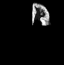
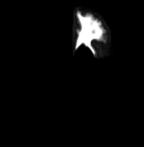
For each case from previous manually segmented 1.5T scans (Nakamura et al, 2007), binary label maps for the leaves (BG,ltgm1-ltgm4, rtgm1-rtgm4, subgm, subwm and CSF) to be segmented were obtained. The manually segmented scans consisted of a single LTWM and RTWM region. However, over multiple experiments it was found that the segmentation works best with no left-right misclassification and between the different GM regions, when WM atlases are given as those closest to a particular GM region as opposed to providing a single left or right WM atlas for the respective left or right GM regions. For example, providing ltwm1 for gm1 region and ltwm2 for gm2 region worked better than providing a ltwm atlas common to ltgm1, ltgm2, ltgm3, ltgm4. Thus using distance transform the WM atlases were split into ltwm1, ltwm2, rtwm1 rtwm2 etc. depending on which gm region the WM was closest to. Hence 8 regions ltwm1-ltwm4 and rtwm1-rtwm4 were obtained from the single LTWM and RTWM region in the manually segmented scan.
Initially, all these label maps were respectively affine transformed to a pre-determined case. A diffeomorphic registration algorithm (Vercauteren et al, 2008) was applied and this produced warps of all the regions for all the cases. The warps were applied to the original images and all the images for respective regions are aligned in a final atlas space. Probability maps are then determined by averaging the images for respective regions i.e. BG, ltgm1, ltgm2, CSF etc.
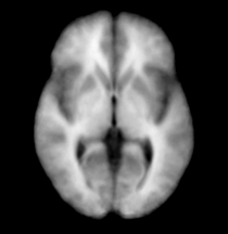
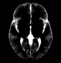
Weighted combined atlases: Left and right classification of the brain typically relies on the atlases since the intensities are similar. Thus if an area on the left side say ltgm1 is not covered adequately by the atlas, the segmentation algorithm puts the next region with the highest probability in the ltgm1 region. Therefore, in order to get an accurate segmentation and to prevent left and right mis-classification, the atlases were weighted and combined for each leaf. For example, for ltgm1 the ltgm1 atlas was weighted by 0.9 and the ltwm1 atlas was weighted by 0.1 and then summed up. Thus in this way, for ltgm1 the atlas covers even the white matter region except that the probability of finding grey matter is lower. The opposite if done for ltwm1 i.e. the ltwm1 atlas is weighted by 0.9 and ltgm1 is weighted by 0.1 and then summed up. These weighted combined atlases provide a much accurate segmentation.
|
|
|
|
| Template (T1) | CSF | Left GM1 (LTGM1) | Left WM1 (LTWM1) |
Result
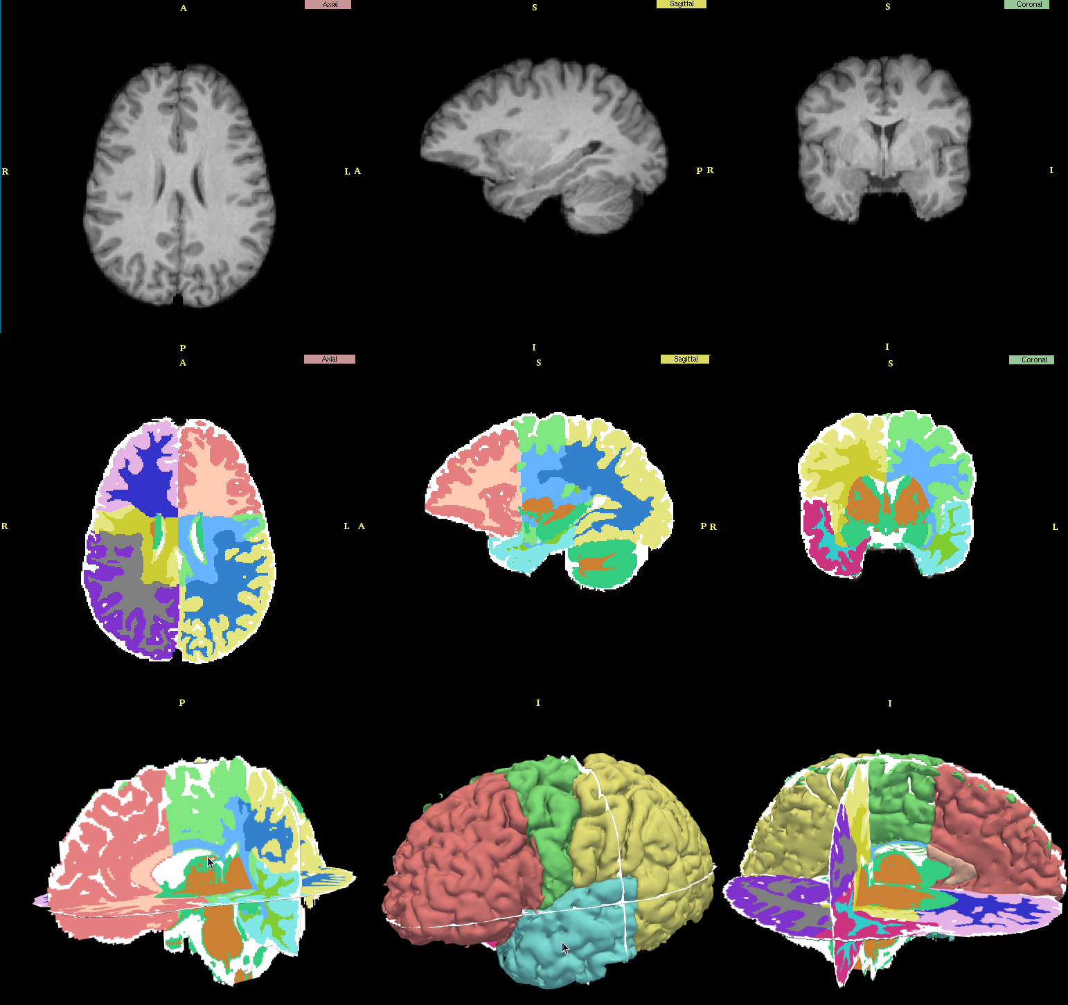
|
| Row 1: Original T1 scans, Row 2: Automatic segmentation, Row 3: Scan in 3D view. |
Collaborators
Padmapriya Srinivasan and Sylvain Bouix (PNL-BWH)
Acknowledgment
The construction of the pipeline was supported by funding from NIH NCRR 2P41RR013218 Supplement.
Citations
- Tustison NJ, Avants BB, Cook PA, Zheng Y, Egan A, Yushkevich PA, Gee JC N4ITK: Improved N3 Bias Correction, IEEE Trans Med Imag, 2010
- Pohl K, Bouix S, Nakamura M, Rohlfing T, McCarley R, Kikinis R, Grimson W, Shenton M, Wells W. A Hierarchical Algorithm for MR Brain Image Parcellation. IEEE Transactions on Medical Imaging. 2007 Sept;26(9):1201-1212.
- S. Warfield, J. Rexilius, P. Huppi, T. Inder, E. Miller, W. Wells, G. Zientara, F. Jolesz, and R. Kikinis, “A binary entropy measure to assess nonrigid registration algorithms,” in MICCAI, LNCS, pp. 266–274, Springer, October 2001.
- Johnson H.J., Harris G., Williams K. BRAINSFit: Mutual Information Registrations of Whole-Brain 3D Images, Using the Insight Toolkit, The Insight Journal, July 2007
- M. Nakamura, D. F. Salisbury, Y. Hirayasu, S. Bouix, K. Pohl, T. Yoshida, M. Koo, M. Koo, R. McCarley. Neocortical Gray Matter Volume in First-Episode Schizophrenia and First-Episode Affective Psychosis: A Cross-Sectional and Longitudinal MRI Study. Biological Psychiatry .Volume 62, Number 7, Pages 773-783. 2007
- T. Vercauteren, X. Pennec, A. Perchant, N. Ayache. Symmetric Log-Domain Diffeomorphic Registration: A Demons-based Approach. MICCAI 2008
- M. Ono, S. Kubik, C.D. Abernathey. Atlas of the Cerebral Sulci. New York: Thieme Medical Publishers. 1990
- Y. Hirayasu, M.E. Shenton, D.F. Salisbury, R.W. McCarley. Hippocampal and superior temporal gyrus volume in first-episode schizophrenia. Arch Gen Psychiatry 2000;57:618–619.