Difference between revisions of "Coordinate systems"
Tag: 2017 source edit |
|||
| (25 intermediate revisions by 4 users not shown) | |||
| Line 1: | Line 1: | ||
| + | |||
| + | {{documentation/banner|text=[https://slicer.readthedocs.io/en/latest/user_guide/coordinate_systems.html For the latest version of this page, visit the read-the-docs.]}} | ||
| + | |||
=Introduction= | =Introduction= | ||
| − | One of the | + | One of the issues while dealing with medical images and applications are the differences between the coordinate systems. There are three coordinate systems commonly used in imaging applications: a difference can be made between the '''world''', '''anatomical''' and the '''image coordinate system'''. |
| + | |||
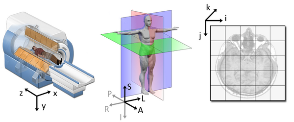
| + | The following figure illustrates the three spaces and their corresponding axes: | ||
| + | [[Image:coordinate_sytems.png| 600px | center]] | ||
| + | |||
| + | |||
| + | Each coordinate system serves one purpose and represents their data in different ways. | ||
| + | |||
| + | Anatomy image based on [http://www.my-ms.org/mri_plane_math.htm image shared by the My MS organization]. | ||
| + | |||
| + | Note that Chand John of Stanford created a [https://www.na-mic.org/w/img_auth.php/3/3f/Coordinate_Systems_Demystified.ppt detailed powerpoint presentation about the way coordinates are handled in Slicer]. | ||
| + | |||
| + | ==World coordinate system== | ||
| + | The world coordinate system is typically a Cartesian coordinate system in which a model (e.g. a MRI scanner or a patient) is positioned. Every model has its own coordinate system but there is only one world coordinate system to define the position and orientation of each model. | ||
| + | |||
| + | ==Anatomical coordinate system== | ||
| + | The most important model coordinate system for medical imaging techniques is the anatomical space (also called patient coordinate system). This space consists of three planes to describe the standard anatomical position of a human: | ||
| + | * the ''axial plane'' is parallel to the ground and separates the head (Superior) from the feet (Inferior) | ||
| + | * the ''coronal plane'' is perpendicular to the ground and separates the front from (Anterior) the back (Posterior) | ||
| + | * the ''sagittal plane'' separates the Left from the Right | ||
| + | From these planes it follows that all axes have their notation in a positive direction (e.g. the negative Superior axis is represented by the Inferior axis). | ||
| + | |||
| + | The anatomical coordinate system is a continuous three-dimensional space in which an image has been sampled. In neuroimaging, it is common to define this space with respect to the human whose brain is being scanned. Hence the 3D basis is defined along the anatomical axes of anterior-posterior, inferior-superior, and left-right. | ||
| + | |||
| + | However different medical applications use different definitions of this 3D basis. Most common are the following bases: | ||
| + | * LPS (Left, Posterior, Superior) is used in DICOM images and by the ITK toolkit | ||
| + | <div style="text-align: center;"> | ||
| + | <math> LPS = \begin{Bmatrix} | ||
| + | \text{from right towards left} \\ | ||
| + | \text{from anterior towards posterior} \\ | ||
| + | \text{from inferior towards superior} | ||
| + | \end{Bmatrix} | ||
| + | </math> | ||
| + | </div> | ||
| + | * RAS (Right, Anterior, Superior) is similar to LPS with the first two axes flipped and used by 3D Slicer | ||
| + | <div style="text-align: center;"> | ||
| + | <math> RAS = \begin{Bmatrix} | ||
| + | \text{from left towards right} \\ | ||
| + | \text{from posterior towards anterior} \\ | ||
| + | \text{from inferior towards superior} | ||
| + | \end{Bmatrix} | ||
| + | </math> | ||
| + | </div> | ||
| + | Both bases are equally useful and logical. It is just necessary to know to which basis an image is referenced. | ||
| + | |||
| + | ==Image coordinate system== | ||
| + | The image coordinate system describes how an image was acquired with respect to the anatomy. Medical scanners create regular, rectangular arrays of points and cells which start at the upper left corner. The ''i'' axis increases to the right, the ''j'' axis to the bottom and the ''k'' axis backwards. | ||
| + | |||
| + | In addition to the intensity value of each voxel ''(i j k)'' the origin and spacing of the anatomical coordinates are stored too. | ||
| + | * The origin represents the position of the first voxel (0,0,0) in the anatomical coordinate system, e.g. (100mm, 50mm, -25mm) | ||
| + | * The spacing specifies the distance between voxels along each axis, e.g. (1.5mm, 0.5mm, 0.5mm) | ||
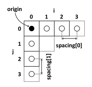
| + | The following 2D example shows the meaning of origin and spacing: | ||
| + | [[Image:Image_Coordinats.png| 300px | center]] | ||
| + | |||
| + | Using the origin and spacing, the corresponding position of each (image coordinate) voxel in anatomical coordinates can be calculated. | ||
| + | |||
| + | =Image transformation= | ||
| + | The transformation from an image space vector <math>(i\;j\;k)'</math> to an anatomical space vector <math>\vec{x}</math> is an affine transformation, consists of a linear transformation <math>\displaystyle A</math> followed by a translation <math>\vec{t}</math>. | ||
| + | <div style="text-align: center;"> | ||
| + | <math> | ||
| + | \vec{x} = A \begin{pmatrix} i & j & k \end{pmatrix}' + \vec{t} | ||
| + | </math> | ||
| + | </div> | ||
| + | |||
| + | The transformation matrix <math>\displaystyle A</math> is a <math>3\,\times\,3</math> matrix and carries all information about space directions and axis scaling. | ||
| + | |||
| + | <math>\vec{t}</math> is a <math>3\,\times\,1</math> vector and contains information about the geometric position of the first voxel. | ||
| + | <div style="text-align: center;"> | ||
| + | <math> | ||
| + | \begin{pmatrix} x_1 \\ x_2 \\ x_3 \end{pmatrix} = | ||
| + | \begin{pmatrix} A_{11} & A_{12} & A_{13} \\ A_{21} & A_{22} & A_{23} \\ A_{31} & A_{32} & A_{33} \end{pmatrix} | ||
| + | \begin{pmatrix} i \\ j \\ k \end{pmatrix} + \begin{pmatrix} t_1 \\ t_2 \\ t_3 \end{pmatrix} | ||
| + | </math> | ||
| + | </div> | ||
| + | |||
| + | The last equation shows that the linear transformation is performed by a matrix multiplication and the translation by a vector addition. To represent both, the transformation and the translation, by a matrix multiplication an augmented matrix must be used. This technique requires that the matrix <math>\displaystyle A</math> is augmented with an extra row of zeros at the bottom, an extra column-the translation vector-to the right, and a '1' in the lower right corner. Additionally all vectors have to be written as homogeneous coordinates, which means that a '1' is augmented at the end. | ||
| + | <div style="text-align: center;"> | ||
| + | <math> | ||
| + | \begin{pmatrix} x_1 \\ x_2 \\ x_3 \\ 1 \end{pmatrix} = | ||
| + | \begin{pmatrix} A_{11} & A_{12} & A_{13} & t_1 \\ A_{21} & A_{22} & A_{23} & t_2 \\ | ||
| + | A_{31} & A_{32} & A_{33} & t_3 \\ 0 & 0 & 0 & 1 \end{pmatrix} | ||
| + | \begin{pmatrix} i \\ j \\ k \\ 1 \end{pmatrix} | ||
| + | </math> | ||
| + | </div> | ||
| + | |||
| + | Depending on the used anatomical space (LPS or RAS) the <math>4\,\times\,4</math> matrix is called '''IJKtoLPS'''- or '''IJKtoRAS'''-matrix, because it represents the transformation from IJK to LPS or RAS. | ||
| + | |||
| + | =2D example or calculating an ''IJtoLS''-matrix= | ||
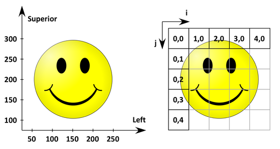
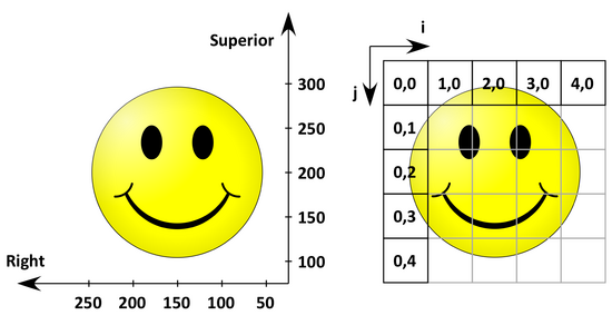
| + | The following figure shows the anatomical space with a L(P)S basis on the left and the corresponding image coordinates on the right. | ||
| + | [[Image:IJtoLS.png| 550px | center]] | ||
| + | |||
| + | The origin (the coordinates of the first 'pixel' in anatomical space) is ''(50 mm, 300 mm)'' and the spacing (the distance between two pixels) is ''(50 mm, 50 mm)''. | ||
| + | |||
| + | As this is a 2D example <math>\displaystyle A</math> is a <math>2\,\times\,2</math> matrix and <math>\vec{t}</math> a <math>2\,\times\,1</math> vector. Therefore the equation of the affine transformation is: | ||
| + | <div style="text-align: center;"> | ||
| + | <math> | ||
| + | \begin{pmatrix} L \\ S \\ 1 \end{pmatrix} = | ||
| + | \begin{pmatrix} A_{11} & A_{12} & t_1 \\ A_{21} & A_{22} & t_2 \\ 0 & 0 & 1 \end{pmatrix} | ||
| + | \begin{pmatrix} i \\ j \\ 1 \end{pmatrix} | ||
| + | </math> | ||
| + | </div> | ||
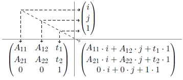
| + | By multiplying the '''IJtoLS'''-matrix and the vector of the right side, the following product will be obtained: | ||
| + | [[Image:Matrix_multiplication.png| center]] | ||
| + | |||
| + | The last equation and the matrix product show that a total of 6 unknown variables <math>\displaystyle(A_{11}, A_{12}, A_{21}, A_{22}, t_1, t_2)</math> have to be determined. The knowledge of origin and spacing however allows the following relations between image and anatomical space: | ||
| + | <div style="text-align: center;"> | ||
| + | <math> | ||
| + | \begin{pmatrix} L \\ S \end{pmatrix} \equiv \begin{pmatrix} i \\ j \end{pmatrix} \qquad | ||
| + | \begin{pmatrix} 50 \\ 300 \end{pmatrix} \equiv \begin{pmatrix} 0 \\ 0 \end{pmatrix} \qquad | ||
| + | \begin{pmatrix} 100 \\ 300 \end{pmatrix} \equiv \begin{pmatrix} 1 \\ 0 \end{pmatrix} \qquad | ||
| + | \begin{pmatrix} 50 \\ 250 \end{pmatrix} \equiv \begin{pmatrix} 0 \\ 1 \end{pmatrix} \qquad \dots | ||
| + | </math> | ||
| + | </div> | ||
| + | |||
| + | Thus, at least six equations can be derived: | ||
| + | <div style="text-align: center;"> | ||
| + | <math>50 = A_{11} \cdot 0 + A_{12} \cdot 0 + t_1 \cdot 1 </math> | ||
| + | |||
| + | <math>300 = A_{21} \cdot 0 + A_{22} \cdot 0 + t_2 \cdot 1 </math> | ||
| + | |||
| + | <math>100 = A_{11} \cdot 1 + A_{12} \cdot 0 + t_1 \cdot 1 </math> | ||
| + | |||
| + | <math>300 = A_{21} \cdot 1 + A_{22} \cdot 0 + t_2 \cdot 1 </math> | ||
| + | |||
| + | <math>50 = A_{11} \cdot 0 + A_{12} \cdot 1 + t_1 \cdot 1 </math> | ||
| + | |||
| + | <math>250 = A_{21} \cdot 0 + A_{22} \cdot 1 + t_2 \cdot 1 </math> | ||
| + | </div> | ||
| + | |||
| + | As mentioned above, the translation <math>\vec{t}</math> contains the information about the geometric position of the first pixel and is therefore equivalent to the origin. This result is also confirmed by the first equations. | ||
| + | |||
| + | The solution of the other equations leads to the following '''IJtoLS'''-matrix: | ||
| + | <div style="text-align: center;"> | ||
| + | <math> | ||
| + | IJtoLS = | ||
| + | \begin{pmatrix} 50 & 0 & 50 \\ 0 & -50 & 300 \\ 0 & 0 & 1 \end{pmatrix} | ||
| + | </math> | ||
| + | </div> | ||
| + | |||
| + | In the event that a R(A)S basis was used, just the left and anterior axis of the anatomical space are flipped, and the image coordinate system appears in the same way as in the L(P)S case. | ||
| + | [[Image:IJtoRS.png| 550px | center]] | ||
| + | |||
| + | For this 2D example the '''IJtoRS'''-matrix would be: | ||
| + | <div style="text-align: center;"> | ||
| + | <math> | ||
| + | IJtoRS = | ||
| + | \begin{pmatrix} -50 & 0 & 250 \\ 0 & -50 & 300 \\ 0 & 0 & 1 \end{pmatrix} | ||
| + | </math> | ||
| + | </div> | ||
| + | |||
| + | This matrix looks very similar to the '''IJtoLS'''-matrix with 2 differences: | ||
| + | * The translation <math>\vec{t}</math> has changed because of another origin | ||
| + | * The right axis is flipped, so the first column of the '''IJtoRS'''-matrix has just an inverted sign | ||
| + | |||
| + | = Relations to other software / conventions = | ||
| − | + | == Using MATLAB to map Slicer RAS coordinates (e.g. fiducials) to voxel space of a NIfTI Image == | |
| − | |||
| − | + | To extract the "voxel to world" transformation matrix from the NIFTI file's header (entry: qto_xyz:1-4 ) in Matlab: | |
| − | |||
| − | |||
| − | |||
| − | |||
| − | |||
| − | |||
| − | |||
| − | = | + | d=inv(M) *[ R A S 1 ]' |
| − | |||
| − | + | where M is the matrix and R A S are coordinates in Slicer, then d gives a vector of voxel coordinates. | |
| − | |||
| − | |||
| + | (Solution courtesy of András Jakab, University of Debrecen) | ||
| − | = | + | =References= |
| − | + | * http://people.cs.uchicago.edu/~glk/unlinked/nrrd-iomf.pdf | |
| + | * http://www.grahamwideman.com/gw/brain/orientation/orientterms.htm | ||
| + | * http://nifti.nimh.nih.gov/nifti-1/documentation/faq | ||
| + | * http://teem.sourceforge.net/nrrd/format.html | ||
| + | * [http://medical.nema.org/dicom/2013/output/chtml/part03/sect_C.7.html#sect_C.7.6.2.1.1 DICOM 2013 PS3.3 Image Position and Image Orientation] | ||
Latest revision as of 14:48, 26 July 2023
Home < Coordinate systems|
For the latest version of this page, visit the read-the-docs. |
Contents
Introduction
One of the issues while dealing with medical images and applications are the differences between the coordinate systems. There are three coordinate systems commonly used in imaging applications: a difference can be made between the world, anatomical and the image coordinate system.
The following figure illustrates the three spaces and their corresponding axes:
Each coordinate system serves one purpose and represents their data in different ways.
Anatomy image based on image shared by the My MS organization.
Note that Chand John of Stanford created a detailed powerpoint presentation about the way coordinates are handled in Slicer.
World coordinate system
The world coordinate system is typically a Cartesian coordinate system in which a model (e.g. a MRI scanner or a patient) is positioned. Every model has its own coordinate system but there is only one world coordinate system to define the position and orientation of each model.
Anatomical coordinate system
The most important model coordinate system for medical imaging techniques is the anatomical space (also called patient coordinate system). This space consists of three planes to describe the standard anatomical position of a human:
- the axial plane is parallel to the ground and separates the head (Superior) from the feet (Inferior)
- the coronal plane is perpendicular to the ground and separates the front from (Anterior) the back (Posterior)
- the sagittal plane separates the Left from the Right
From these planes it follows that all axes have their notation in a positive direction (e.g. the negative Superior axis is represented by the Inferior axis).
The anatomical coordinate system is a continuous three-dimensional space in which an image has been sampled. In neuroimaging, it is common to define this space with respect to the human whose brain is being scanned. Hence the 3D basis is defined along the anatomical axes of anterior-posterior, inferior-superior, and left-right.
However different medical applications use different definitions of this 3D basis. Most common are the following bases:
- LPS (Left, Posterior, Superior) is used in DICOM images and by the ITK toolkit
[math] LPS = \begin{Bmatrix} \text{from right towards left} \\ \text{from anterior towards posterior} \\ \text{from inferior towards superior} \end{Bmatrix} [/math]
- RAS (Right, Anterior, Superior) is similar to LPS with the first two axes flipped and used by 3D Slicer
[math] RAS = \begin{Bmatrix} \text{from left towards right} \\ \text{from posterior towards anterior} \\ \text{from inferior towards superior} \end{Bmatrix} [/math]
Both bases are equally useful and logical. It is just necessary to know to which basis an image is referenced.
Image coordinate system
The image coordinate system describes how an image was acquired with respect to the anatomy. Medical scanners create regular, rectangular arrays of points and cells which start at the upper left corner. The i axis increases to the right, the j axis to the bottom and the k axis backwards.
In addition to the intensity value of each voxel (i j k) the origin and spacing of the anatomical coordinates are stored too.
- The origin represents the position of the first voxel (0,0,0) in the anatomical coordinate system, e.g. (100mm, 50mm, -25mm)
- The spacing specifies the distance between voxels along each axis, e.g. (1.5mm, 0.5mm, 0.5mm)
The following 2D example shows the meaning of origin and spacing:
Using the origin and spacing, the corresponding position of each (image coordinate) voxel in anatomical coordinates can be calculated.
Image transformation
The transformation from an image space vector [math](i\;j\;k)'[/math] to an anatomical space vector [math]\vec{x}[/math] is an affine transformation, consists of a linear transformation [math]\displaystyle A[/math] followed by a translation [math]\vec{t}[/math].
[math] \vec{x} = A \begin{pmatrix} i & j & k \end{pmatrix}' + \vec{t} [/math]
The transformation matrix [math]\displaystyle A[/math] is a [math]3\,\times\,3[/math] matrix and carries all information about space directions and axis scaling.
[math]\vec{t}[/math] is a [math]3\,\times\,1[/math] vector and contains information about the geometric position of the first voxel.
[math] \begin{pmatrix} x_1 \\ x_2 \\ x_3 \end{pmatrix} = \begin{pmatrix} A_{11} & A_{12} & A_{13} \\ A_{21} & A_{22} & A_{23} \\ A_{31} & A_{32} & A_{33} \end{pmatrix} \begin{pmatrix} i \\ j \\ k \end{pmatrix} + \begin{pmatrix} t_1 \\ t_2 \\ t_3 \end{pmatrix} [/math]
The last equation shows that the linear transformation is performed by a matrix multiplication and the translation by a vector addition. To represent both, the transformation and the translation, by a matrix multiplication an augmented matrix must be used. This technique requires that the matrix [math]\displaystyle A[/math] is augmented with an extra row of zeros at the bottom, an extra column-the translation vector-to the right, and a '1' in the lower right corner. Additionally all vectors have to be written as homogeneous coordinates, which means that a '1' is augmented at the end.
[math] \begin{pmatrix} x_1 \\ x_2 \\ x_3 \\ 1 \end{pmatrix} = \begin{pmatrix} A_{11} & A_{12} & A_{13} & t_1 \\ A_{21} & A_{22} & A_{23} & t_2 \\ A_{31} & A_{32} & A_{33} & t_3 \\ 0 & 0 & 0 & 1 \end{pmatrix} \begin{pmatrix} i \\ j \\ k \\ 1 \end{pmatrix} [/math]
Depending on the used anatomical space (LPS or RAS) the [math]4\,\times\,4[/math] matrix is called IJKtoLPS- or IJKtoRAS-matrix, because it represents the transformation from IJK to LPS or RAS.
2D example or calculating an IJtoLS-matrix
The following figure shows the anatomical space with a L(P)S basis on the left and the corresponding image coordinates on the right.
The origin (the coordinates of the first 'pixel' in anatomical space) is (50 mm, 300 mm) and the spacing (the distance between two pixels) is (50 mm, 50 mm).
As this is a 2D example [math]\displaystyle A[/math] is a [math]2\,\times\,2[/math] matrix and [math]\vec{t}[/math] a [math]2\,\times\,1[/math] vector. Therefore the equation of the affine transformation is:
[math] \begin{pmatrix} L \\ S \\ 1 \end{pmatrix} = \begin{pmatrix} A_{11} & A_{12} & t_1 \\ A_{21} & A_{22} & t_2 \\ 0 & 0 & 1 \end{pmatrix} \begin{pmatrix} i \\ j \\ 1 \end{pmatrix} [/math]
By multiplying the IJtoLS-matrix and the vector of the right side, the following product will be obtained:
The last equation and the matrix product show that a total of 6 unknown variables [math]\displaystyle(A_{11}, A_{12}, A_{21}, A_{22}, t_1, t_2)[/math] have to be determined. The knowledge of origin and spacing however allows the following relations between image and anatomical space:
[math] \begin{pmatrix} L \\ S \end{pmatrix} \equiv \begin{pmatrix} i \\ j \end{pmatrix} \qquad \begin{pmatrix} 50 \\ 300 \end{pmatrix} \equiv \begin{pmatrix} 0 \\ 0 \end{pmatrix} \qquad \begin{pmatrix} 100 \\ 300 \end{pmatrix} \equiv \begin{pmatrix} 1 \\ 0 \end{pmatrix} \qquad \begin{pmatrix} 50 \\ 250 \end{pmatrix} \equiv \begin{pmatrix} 0 \\ 1 \end{pmatrix} \qquad \dots [/math]
Thus, at least six equations can be derived:
[math]50 = A_{11} \cdot 0 + A_{12} \cdot 0 + t_1 \cdot 1 [/math]
[math]300 = A_{21} \cdot 0 + A_{22} \cdot 0 + t_2 \cdot 1 [/math]
[math]100 = A_{11} \cdot 1 + A_{12} \cdot 0 + t_1 \cdot 1 [/math]
[math]300 = A_{21} \cdot 1 + A_{22} \cdot 0 + t_2 \cdot 1 [/math]
[math]50 = A_{11} \cdot 0 + A_{12} \cdot 1 + t_1 \cdot 1 [/math]
[math]250 = A_{21} \cdot 0 + A_{22} \cdot 1 + t_2 \cdot 1 [/math]
As mentioned above, the translation [math]\vec{t}[/math] contains the information about the geometric position of the first pixel and is therefore equivalent to the origin. This result is also confirmed by the first equations.
The solution of the other equations leads to the following IJtoLS-matrix:
[math] IJtoLS = \begin{pmatrix} 50 & 0 & 50 \\ 0 & -50 & 300 \\ 0 & 0 & 1 \end{pmatrix} [/math]
In the event that a R(A)S basis was used, just the left and anterior axis of the anatomical space are flipped, and the image coordinate system appears in the same way as in the L(P)S case.
For this 2D example the IJtoRS-matrix would be:
[math] IJtoRS = \begin{pmatrix} -50 & 0 & 250 \\ 0 & -50 & 300 \\ 0 & 0 & 1 \end{pmatrix} [/math]
This matrix looks very similar to the IJtoLS-matrix with 2 differences:
- The translation [math]\vec{t}[/math] has changed because of another origin
- The right axis is flipped, so the first column of the IJtoRS-matrix has just an inverted sign
Relations to other software / conventions
Using MATLAB to map Slicer RAS coordinates (e.g. fiducials) to voxel space of a NIfTI Image
To extract the "voxel to world" transformation matrix from the NIFTI file's header (entry: qto_xyz:1-4 ) in Matlab:
d=inv(M) *[ R A S 1 ]'
where M is the matrix and R A S are coordinates in Slicer, then d gives a vector of voxel coordinates.
(Solution courtesy of András Jakab, University of Debrecen)
