Documentation/Labs/Slicer Visualization module

Overview

This is a page introducing the Slicer Connectome Visualization project for adding new visualization extensions into 3DSlicer.

What do we want to visualize?
Visualizations are based on symmetric and normalized matrices (AAL or Destrieux)) with connectivity values that may be obtained from diffusion connectivity or resting state connectivity studies (region-to-region values).
The matrices represent a graph, where the edges are the connectivity values and the nodes are brain regions.

What do we mean by connectome?
The mapping of all neural connections within the brain is what we call a connectome.
Each connection is defined by its strength (visually it represents the thickness of the connection between two nodes) and this value is found in the matrices (edge files).

Goal

Implement two different modules into Slicer:

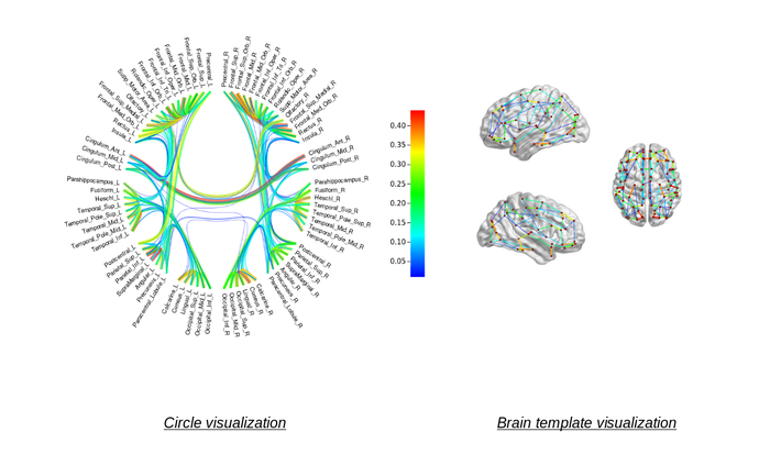
• 2D circle visualization of brain connectome
• 3D volume visualization of brain connectome

Details

The user will have the choice between the 2D and the 3D visualization module. First we will focus on the 3D module and then on the 2D module.

User Inputs (3 ASCII files):

• Volume file
• Node file (and maybe add and option for the user to be able to edit the node characterization ;for example with labels)
• Edge file (could be binary, but we will not impose any constraints on the range)

The Node file and the Edge file will have to be adaptable formats, that is the reason why we want to use ASCII files. The Node file should include information about where the node is located.
The file extension could either be a Landmark Registration format (existing module in Slicer) or a Jason file (including a node description file (x,y,z coordinates and node color index) and a node magnitude file(with just the size of a node)).

Features 3D module:

• Python module (using VTK) and maybe C++
• Implement a 3D visualization tool that is faster than BrainNetViewer and CIVILITY (based on Matlab).
• For each node we could sum the connections and generate 2 files. One disk file (how do I save them on a disk?) and one data structure file (how do I store data in memory?)
• The 3D visualization module should offer the possibility to rotate around the connectome and zoom for more precision.
• Impose a minimum strength on the connectome connections

Features 2D module:

• Use as much Python as we can (VTK) otherwise C++
• Implement a 2D spherical graph visualization (may apply Hierarchical Edge Bundling), using matrices
  

(possible options: vtkMRMLGraphMarkupNode,vtkSlicerGraphRepresentation3D and associated widget (looking at vtkMRMLMarkupsCurveNode, vtkSlicerCurveRepresentation and vtkSlicerCurveWidget))

• Custom graph view representing the associated matrix and define the connection strength by the opacity of the color